For a scalar valued function \(f: \mathbb{R}^n \to \mathbb{R}\), the first order Taylor expansion near some point \(x_0\) gives the best approximating affine function \(p_1: \mathbb{R}^n \to \mathbb{R}\)

Note that the gradient of \(p_1\) at any point \(x\) is the same (since it's an affine map): \(\nabla p_1(x) = \nabla f(x_0)\)

We can give \(p_1\) three geometric interpretations:

1. In the output space \(\mathbb{R}\), for points \(x\) near \(x_0\), the values of \(f\) lie on a \(1\) dimensional affine subspace that is the image of \(p_1(x)\). This geometric interpretation becomes more interesting for a vector valued function \(\mathbf{f}: \mathbb{R}^n \to \mathbb{R}^m\): the values of \(\mathbf{f}\) lie roughly on an affine subspace of \(\mathbb{R}^m\), which is the column space of the \(m \times n\) Jacobian matrix shifted by \(\mathbf{f}(x_0)\).

   This first interpretation comes straight from the definition of differentiability, which is all about locally approximating an arbitrary function by an affine map.

2. In the input space \(\mathbb{R}^n\), if we pick a point \(x_0 \in \textbf{dom }f\), the level set/surface of \(p_1\) at \(f(x_0)\), \(P = \{ x \in \mathbb{R}^n | p_1(x) = f(x_0)\}\), is a hyperplane with the normal vector \(\nabla f(x_0)\) passing through the point \(x_0\). That is, \(P\) is the set of points in \(\mathbb{R}^n\) that satisfy:

   $$ \nabla f(x_0) (x-x_0) =0 $$
   Consider the level set of \(f\) at \(f(x_0)\), \(S = \{ x \in \mathbb{R}^n | f(x) = f(x_0)\}\). In \(\mathbb{R}^2\), \(S\) is a contour line of \(f\), and \(P\) is just a straight line, both passing through \(x_0\). Important facts:
   • \(\nabla f(x_0)\) is the direction of steepest ascent of \(f\) at the point \(x_0 \in S\)
   • \(\nabla f(x_0)\) is perpendicular to \(S\) at the point \(x_0\)
   • \(P\) is tangent to \(S\) at the point \(x_0\)

   

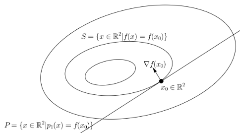
   This second geometric view is used most often in the context of gradient based optimization.

3. In the graph space \(\mathbb{R}^{n+1}\), the graph of \(p_1\) is a hyperplane tangent to the graph of \(f\) at the point \((x_0, f(x_0))\). Recall we define the graph of \(f\) to be the set \(\{ (x, t) | f(x) = t \}\), call it \(G_f\). To find a hyperplane in \(\mathbb{R}^{n+1}\) that is tangent to \(G_f\) at the point \((x_0, f(x_0)) \in G_f\), we introduce a helper function \(F: \mathbb{R}^{n+1} \to \mathbb{R}\), s.t. \(\forall x \in \textbf{dom } f, \forall t \in \mathbb{R}, F(x,t) := f(x) - t\) (think of it as reporting the difference in temperature between the point \(x\) measured by \(f(x)\) and some pre-specified value \(t\)). Then the level set/surface of \(F\) at \(0\) is precisely \(G_f\), and based on the second geometric view, we can find the normal vector to \(G_f\) at \((x_0, f(x_0))\) by evaluating the gradient of \(F\) at \((x_0, f(x_0))\) (which is just another point in its input space):

   $$\nabla F(x_0, f(x_0)) = [ \nabla f(x_0) \quad \frac{\partial F}{\partial t} ] = [ \nabla f(x_0) \quad -1 ] $$
   The hyperplane we're looking for is therefore the set of points \((x,t) \in \mathbb{R}^{n+1}\) that satisfy:
   $$ \nabla F(x_0, f(x_0)) (\begin{bmatrix} x \\ t \end{bmatrix} - \begin{bmatrix} x_0 \\ f(x_0) \end{bmatrix}) = 0 $$
   or simply,
   $$f(x_0) + \nabla f(x_0) (x-x_0) = t$$
   This is precisely the graph of \(p_1\), i.e. the set \(G_p = \{ (x, t) | p_1(x) = t \}\). So we see that the \(G_p\) is tangent to \(G_f\) at the point \((x_0, f(x_0))\), and the vector \([ \nabla f(x_0) \quad -1 ]\) is perpendicular to \(G_f\) at \((x_0, f(x_0))\). Since \(S\) is just a slice of \(G_f\) at the height \(f(x_0)\), similarly \(P\) a slice of \(G_p\) at the same height, the earlier assertion makes geometric sense: \(P\) must be tangent to \(S\) at the point \(x_0\), because the graphs containing them (\(G_f\) and \(G_p\)) are tangent at \((x_0, f(x_0)\).

   This view is most helpful for working with epigraphs of functions.

   For an application, let's consider the geometry of epigraphs for convex functions, based on the last view from graph space. Recall the epigraph of a function \(f: \mathbb{R}^n \to \mathbb{R}\) is a subset of \(\mathbb{R}^{n+1}\), \(\textbf{epi }f := \{ (x, t)| x \in \textbf{dom }f, f(x) \leq t \}\). By the first order condition of convexity, for convex \(f\) we have

   $$\forall x, y \in \textbf{dom }f, f(y) \geq f(x) + \nabla f(x)^\top (y-x) $$
   which says that the first-order Taylor approximation of \(f\) at any point \(x\) is always a global underestimator of the function. This inequality implies:
   $$ \forall (y,t) \in \textbf{epi }f, \quad t \geq f(y) \geq f(x) + \nabla f(x)^\top (y-x) $$
   or
   $$ (y,t) \in \textbf{epi }f \implies [\nabla f(x) \quad -1] (\begin{bmatrix} y \\ t \end{bmatrix} - \begin{bmatrix} x \\ f(x) \end{bmatrix}) \leq 0 $$
   for all choices of \(x\). Geometrically, this says that the hyperplane defined by the normal vector \((∇f(x), −1)\) supports \(\textbf{epi }f\) at the boundary point \((x, f(x))\).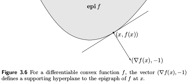

   

References: Vector Calculus p. 165 - p. 168 (esp. example 8 on p. 167) and Convex Optimization p. 76.